Ideas
Your Switches Are Screaming. Nobody's Listening.
Building a real-time AI log analyzer from scratch with a Unix box, a few devices, and zero enterprise software. Here's the actual POC.
Every switch in your network is having a conversation. Right now. It’s spitting out syslog messages at a rate that would make a teenager’s group chat look quiet — interface state changes, spanning-tree recalculations, authentication failures, power supply warnings, fan speed alerts, NTP sync losses, memory allocation errors. Hundreds of messages per minute, per device.
And nobody’s reading them.
Oh sure, they’re going somewhere. Maybe a syslog server that stores them in flat files nobody opens. Maybe a SIEM that indexes them and charges you per gigabyte for the privilege. Maybe they’re hitting the default buffer on the switch itself, silently rolling over and vanishing into the void every 4,096 messages.
But actually understanding them in real time? Correlating that the three switches on floors four, five, and six all went down within the same 90-second window — and that probably means a power issue, not three simultaneous hardware failures? Noticing that your storage array has been creeping up 2% per day and you’ve got about two weeks before it hits the wall?
That’s the stuff that falls through the cracks. Not because the data isn’t there, but because the volume buries the signal so deep that human eyes can’t find it in time.
I’ve been digging into how AI can actually process this firehose in real time, and I found that the answer isn’t one technology — it’s a layered system where each layer does exactly one job. The deeper I went, the more I realized you could build a working proof of concept with a Unix box, a few network devices, and about $0 in software licensing.
Here’s how.
The Two-Brain Problem
The naive approach to “AI-powered log analysis” goes something like this: pipe all your logs into ChatGPT and ask it what’s wrong. And I’ll be honest, for a home lab with three devices, that might actually work. But for anything resembling a real environment — say 200 firewalls and 5,000 switches — you hit a wall immediately.
A busy Cisco switch can generate 50-200 syslog messages per minute under normal conditions. A firewall doing deep packet inspection on a busy link? Easily 500-1,000 messages per minute. Let’s do the math on a modest enterprise:
The Firehose — Typical Enterprise Syslog Volume
════════════════════════════════════════════════

200 firewalls × 500 msg/min    = 100,000 msg/min
5,000 switches × 100 msg/min   = 500,000 msg/min
500 servers × 50 msg/min        = 25,000 msg/min
200 APs × 20 msg/min            = 4,000 msg/min
━━━━━━━━━━━━━━━━━━━━━━━━━━━━━━━━━━━━━━━━━━
Total:                           ~629,000 msg/min
                                 ~10,500 msg/sec
                                 ~900 million msg/day

At an average of 200 tokens per log message:
Token consumption:               ~2.1 billion tokens/day

Claude Sonnet at $3/million input tokens:
Daily cost:                      ~$6,300/day
Monthly cost:                    ~$189,000/month

Just to READ them. Not analyze. Not correlate. Just ingest.
So yeah. Throwing an LLM at raw syslog streams is like hiring a Supreme Court justice to read your junk mail. Technically possible, catastrophically expensive, and a waste of a very capable brain on a very stupid task.
The solution isn’t to avoid AI. It’s to use the right kind of AI at each layer. And this is where it gets interesting, because most of what happens in the first layer isn’t AI at all.
Tier 1: The Mechanical Bouncer
The first layer of any real-time log processing pipeline is pure, old-school, deterministic filtering. No neural networks. No model inference. Just regex, pattern matching, and conditional logic running at wire speed.
This is the part that ChatGPT glossed over when I asked about it, and honestly, it’s the most important part. Because this layer is responsible for reducing 10,000 messages per second down to maybe 10-50 that are actually worth thinking about.
Here’s what Tier 1 actually does:
# Tier 1: Deterministic pre-filter
# This isn't AI. This is a bouncer at the door.

import re
from dataclasses import dataclass
from enum import Enum

class Severity(Enum):
    EMERGENCY = 0    # System unusable
    ALERT = 1        # Immediate action needed
    CRITICAL = 2     # Critical conditions
    ERROR = 3        # Error conditions
    WARNING = 4      # Warning conditions
    NOTICE = 5       # Normal but significant
    INFO = 6         # Informational
    DEBUG = 7        # Debug messages

# Syslog messages follow RFC 5424 format
# <priority>version timestamp hostname app-name procid msgid structured-data msg

NOISE_PATTERNS = [
    r"LINEPROTO-5-UPDOWN.*changed state to up",     # Interface flap recovery
    r"SYS-5-CONFIG_I",                                # Config saved (routine)
    r"SEC_LOGIN-5-LOGIN_SUCCESS",                     # Successful logins (boring)
    r"LINK-3-UPDOWN.*GigabitEthernet0/0/0.*down",   # Known maintenance window
    r"SNMP-3-AUTHFAIL.*public",                       # SNMP community misconfig (known)
    r"CDP-4-NATIVE_VLAN_MISMATCH",                    # Ongoing known issue #4471
    r"STP-2-LOOPGUARD_BLOCK",                         # Handled by STP, self-healing
]

ESCALATION_PATTERNS = [
    (r"PLATFORM-2-PF_PWRSPLY", "power_supply_failure"),
    (r"DUAL-5-NBRCHANGE.*down", "routing_neighbor_down"),
    (r"LINK-3-UPDOWN.*TenGigabit.*down", "uplink_down"),
    (r"SEC_LOGIN-4-LOGIN_FAILED.*repeated", "brute_force_attempt"),
    (r"SYS-2-MALLOCFAIL", "memory_exhaustion"),
    (r"PLATFORM-4-ELEMENT_WARNING.*Temperature", "thermal_warning"),
    (r"FAN-3-FAN_FAILED", "fan_failure"),
    (r"STACKMGR-4-STACK_LINK_CHANGE.*removed", "stack_member_lost"),
]

@dataclass
class FilteredEvent:
    timestamp: str
    source_ip: str
    hostname: str
    severity: Severity
    raw_message: str
    category: str
    escalate_to_ai: bool

def tier1_filter(raw_syslog: str) -> FilteredEvent | None:
    """
    Pure mechanical filtering. No AI. No inference.
    Returns None for messages we don't care about.
    Returns a FilteredEvent for anything that survives.
    """
    # Parse syslog priority to get severity
    severity = parse_severity(raw_syslog)

    # Drop DEBUG and INFO immediately — that's ~70% of all messages
    if severity.value >= Severity.INFO.value:
        return None

    # Drop known noise patterns — another ~20%
    for pattern in NOISE_PATTERNS:
        if re.search(pattern, raw_syslog):
            return None

    # Check for known escalation patterns
    for pattern, category in ESCALATION_PATTERNS:
        if re.search(pattern, raw_syslog):
            return FilteredEvent(
                timestamp=parse_timestamp(raw_syslog),
                source_ip=parse_source(raw_syslog),
                hostname=parse_hostname(raw_syslog),
                severity=severity,
                category=category,
                raw_message=raw_syslog,
                escalate_to_ai=True,
            )

    # Anything else that survived filtering but didn't match
    # an escalation pattern: pass through but don't escalate
    return FilteredEvent(
        timestamp=parse_timestamp(raw_syslog),
        source_ip=parse_source(raw_syslog),
        hostname=parse_hostname(raw_syslog),
        severity=severity,
        category="unclassified",
        raw_message=raw_syslog,
        escalate_to_ai=(severity.value <= Severity.ERROR.value),
    )
Is this AI? No. Not even close. It’s if statements with regex. Your grandma could understand the logic (well, probably not the regex). And yes, it still requires humans to maintain the pattern lists and keep them up to date.
But here’s the thing: this layer isn’t trying to be smart. Its only job is to be fast and to not let the obviously boring stuff through. And it does that job at hundreds of thousands of messages per second on a single CPU core. That speed is the whole point. You’re trading intelligence for throughput, and at this layer, that’s exactly the right trade.
The output of Tier 1 in a typical enterprise? Maybe 50-200 events per minute instead of 10,000 per second. That’s a 99.97% reduction in volume. And now you’ve got something an actual AI can chew on without melting your budget.
“The art of being wise is the art of knowing what to overlook.” — William James
He was talking about philosophy, but he could’ve been talking about syslog.
Tier 2: The Lightweight Machine Learning Models
Here’s where it stops being traditional IT and starts being actual data science. And this is the part that fascinated me the most, because these aren’t LLMs. They’re not language models at all. They don’t understand English. They don’t generate text. They eat numbers and spit out probabilities.
The models that run at this tier are fundamentally different from ChatGPT or Claude. They’re specialized mathematical engines that do one thing exceptionally well: find patterns in numerical data that humans would miss.
Anomaly Detection: The Isolation Forest
Let me explain how an isolation forest works, because it’s beautifully simple once you see it.
Imagine you have a scatter plot of data points. Most of them are clustered together — that’s your “normal.” A few outliers are way off by themselves — those are your anomalies.
An isolation forest builds a bunch of random decision trees. At each node, it picks a random feature and a random split point. Normal data points — the ones in the dense cluster — take many splits to isolate because they have so many neighbors. Anomalous data points — the loners — get isolated quickly because they’re already far from everyone else.
The number of splits needed to isolate a point becomes its “anomaly score.” Few splits = more anomalous. Many splits = more normal.
That’s it. No thresholds. No “alert when CPU > 85%.” The model learns what normal looks like from your actual data and flags anything that doesn’t fit.
# Anomaly detection with Isolation Forest
# This is the ENTIRE model training. Not kidding.

from sklearn.ensemble import IsolationForest
import numpy as np

# Features extracted from your log stream over the past 30 days:
# [hour_of_day, day_of_week, msg_rate_per_min, error_rate,
#  unique_sources, severity_avg, interface_flap_count]

# Collect 30 days of "normal" operation as training data
training_data = np.array([
    # hour, dow, msg_rate, err_rate, sources, sev_avg, flaps
    [  2,    1,   45,       0.02,     12,      5.1,     0  ],  # Typical Tuesday 2am
    [  9,    1,   380,      0.05,     48,      4.8,     2  ],  # Tuesday morning rush
    [ 14,    3,   290,      0.03,     42,      5.0,     1  ],  # Thursday afternoon
    [  2,    6,   850,      0.01,     15,      5.5,     0  ],  # Saturday backup window
    # ... thousands more rows from your actual environment
])

# Train the model. That's literally one line.
model = IsolationForest(
    n_estimators=200,          # Number of trees
    contamination=0.01,        # Expect ~1% of data to be anomalous
    random_state=42,
    n_jobs=-1,                 # Use all CPU cores
)
model.fit(training_data)

# Now, in real time, score each 1-minute window:
def score_current_window(features: np.ndarray) -> float:
    """
    Returns anomaly score. -1 = anomaly, 1 = normal.
    The more negative, the more anomalous.
    """
    score = model.decision_function(features.reshape(1, -1))
    return score[0]

# Example: It's Tuesday at 2am but message rate is 900/min
# The model knows Tuesday 2am is usually 45/min
# Score: -0.34 → ANOMALY
current = np.array([2, 1, 900, 0.15, 38, 3.2, 7])
print(f"Anomaly score: {score_current_window(current)}")
# Output: Anomaly score: -0.34  ← Something's wrong
Notice what just happened. Nobody configured a threshold. Nobody said “alert when message rate exceeds 500.” The model looked at 30 days of your data and figured out that Tuesday at 2 AM usually means 45 messages per minute. When it saw 900, it didn’t compare to a static number — it compared to what your specific network usually does at that specific time on that specific day of the week.
Saturday at 2 AM showing 850 messages? The model knows that’s the backup window. Normal. No alert. But Tuesday at 2 AM showing 900? That’s a 20x deviation from the learned baseline. Fire the alert.
This is why these models beat static thresholds: they understand context. And they do it without understanding a single word of English.
Time Series Forecasting: Seeing the Future
Remember the storage example? Disk usage climbing 2% per day, currently at 88%? A static threshold at 90% gives you one day of warning. A time series model gives you two weeks.
# Time series forecasting with Prophet
# Predict when your storage will hit 100%

from prophet import Prophet
import pandas as pd

# Historical storage utilization data (daily readings)
df = pd.DataFrame({
    'ds': pd.date_range('2026-01-01', periods=60, freq='D'),
    'y': [
        # 60 days of slowly climbing storage
        52, 52, 53, 53, 54, 54, 55, 55, 56, 56,
        57, 57, 58, 58, 59, 60, 60, 61, 61, 62,
        63, 63, 64, 64, 65, 66, 66, 67, 68, 68,
        69, 70, 70, 71, 72, 72, 73, 74, 74, 75,
        76, 76, 77, 78, 78, 79, 80, 80, 81, 82,
        83, 83, 84, 85, 85, 86, 87, 87, 88, 89,
    ]
})

# Train the model
model = Prophet(
    daily_seasonality=False,
    weekly_seasonality=True,
    yearly_seasonality=False,
)
model.fit(df)

# Forecast 30 days ahead
future = model.make_future_dataframe(periods=30)
forecast = model.predict(future)

# Find when utilization crosses 95%
critical = forecast[forecast['yhat'] >= 95].iloc[0]
print(f"Storage will hit 95% around: {critical['ds'].date()}")
print(f"Days until critical: {(critical['ds'] - pd.Timestamp.now()).days}")

# Output: Storage will hit 95% around: 2026-03-16
# Output: Days until critical: 7
Prophet (from Meta) is free, runs on a single CPU, and doesn’t need a GPU. It handles weekly seasonality automatically — so if your storage always spikes on Fridays because of weekly reports and drops slightly on weekends when temp files get cleaned, the model accounts for that.
But the model itself doesn’t tell you anything. It outputs a number. That’s it. A probability curve of future values. Something else needs to take that number and decide it’s worth telling a human about.
Classification: Is This a Real Threat or Just Tuesday?
Here’s a scenario: your firewall logs show 47 failed SSH attempts from an IP address in the last hour. Is it a brute force attack, or is it Dave from accounting who forgot his password again?
A gradient-boosted classifier can learn the difference:
# XGBoost classifier: real threat vs. noise
import xgboost as xgb
import numpy as np

# Features for each "suspicious event" cluster:
# [attempts_per_hour, unique_usernames_tried, unique_source_ips,
#  time_of_day, is_weekend, source_is_internal, geo_distance_km,
#  has_successful_login_history, password_complexity_score]

# Labeled training data from historical incidents
X_train = np.array([
    # Dave forgot his password (noise)
    [12,  1, 1, 9,  0, 1,   0, 1, 7],
    [8,   1, 1, 14, 0, 1,   0, 1, 6],
    [15,  1, 1, 10, 0, 1,   0, 1, 8],
    # Actual brute force attacks (threat)
    [847, 23, 1, 3,  1, 0, 8400, 0, 2],
    [412, 15, 3, 4,  0, 0, 6200, 0, 3],
    [1200, 1, 1, 2,  1, 0, 9100, 0, 1],
    # Credential stuffing (threat)
    [89,  89, 1, 22, 0, 0, 4500, 0, 5],
    [156, 156, 2, 1, 1, 0, 7800, 0, 4],
])
y_train = np.array([0, 0, 0, 1, 1, 1, 1, 1])  # 0=noise, 1=threat

model = xgb.XGBClassifier(
    n_estimators=100,
    max_depth=4,
    learning_rate=0.1,
)
model.fit(X_train, y_train)

# Real-time classification
def classify_event(features):
    proba = model.predict_proba(features.reshape(1, -1))[0]
    return {
        'is_threat': bool(proba[1] > 0.7),
        'confidence': float(proba[1]),
        'label': 'threat' if proba[1] > 0.7 else 'noise',
    }

# New event: 47 attempts, 1 username, internal IP, Monday 9am
event = np.array([47, 1, 1, 9, 0, 1, 0, 1, 7])
result = classify_event(event)
# Output: {'is_threat': False, 'confidence': 0.12, 'label': 'noise'}
# → It's Dave again.
Notice: three completely different model types (isolation forest, Prophet, XGBoost), each handling a different kind of question, all running on the same filtered event stream. They don’t interfere with each other. They don’t even know the other models exist. They’re each independently consuming events and producing scores.
Tier 3: The LLM — The Brains of the Operation
Now — finally — we get to the large language model. But its job is different from what you might expect. The LLM doesn’t read raw logs. It doesn’t process 10,000 messages per second. It gets maybe 10-50 events per minute that have already been pre-filtered (Tier 1) and scored by specialized models (Tier 2).
The LLM’s job is the human-facing part:
-
Correlation: “Three switches went down on adjacent floors within 90 seconds. The ML models flagged each one independently. I’m putting them together and telling you this looks like a localized power or cabling event.”
-
Natural language explanation: “Storage on nas-01 has been climbing 2% daily for 40 days. The time-series model predicts you’ll hit 95% by March 16th. At current growth rates, you’ll be completely full by March 22nd.”
-
Recommended actions: “Based on the thermal warning pattern on core-sw-03 and the fact that you replaced a fan module on this exact model last quarter, I’d suggest checking the fan tray. Here’s the part number.”
-
Historical context: “This is the third time Building B has had this exact failure pattern on a Monday morning. The previous two times it was the UPS doing a self-test under load.”
# Tier 3: LLM integration for human-facing analysis
# This is where the expensive brain gets used — sparingly

import json
from anthropic import Anthropic

client = Anthropic()

def generate_analysis(events: list[dict], ml_scores: dict) -> str:
    """
    Takes pre-filtered events + ML model outputs
    and generates human-readable analysis.
    Called maybe 10-50 times per minute, not 10,000/sec.
    """
    context = {
        "events": events,
        "anomaly_scores": ml_scores.get("anomaly", {}),
        "forecasts": ml_scores.get("forecast", {}),
        "classifications": ml_scores.get("classification", {}),
        "topology": get_network_topology(),  # Cached, updated hourly
        "recent_changes": get_recent_changes(hours=24),
    }

    response = client.messages.create(
        model="claude-haiku-4-5-20251001",  # Fast + cheap for ops analysis
        max_tokens=1024,
        system="""You are a senior network engineer analyzing pre-processed
        infrastructure events. You receive events that have already been
        filtered for significance and scored by ML models for anomaly
        detection, forecasting, and threat classification.

        Your job:
        1. Correlate related events across devices and time
        2. Explain what's happening in plain English
        3. Assess severity and urgency
        4. Recommend specific actions
        5. Reference any relevant historical patterns

        Be direct. No filler. Lead with the most critical finding.""",
        messages=[{
            "role": "user",
            "content": f"Analyze these infrastructure events:\n{json.dumps(context, indent=2)}"
        }]
    )

    return response.content[0].text
Cost at this tier: If you’re processing 50 events/minute through Claude Haiku with ~500 tokens each exchange, that’s about $0.50/day. Not $189,000/month. Because the mechanical bouncer and the ML models already did 99.97% of the work.
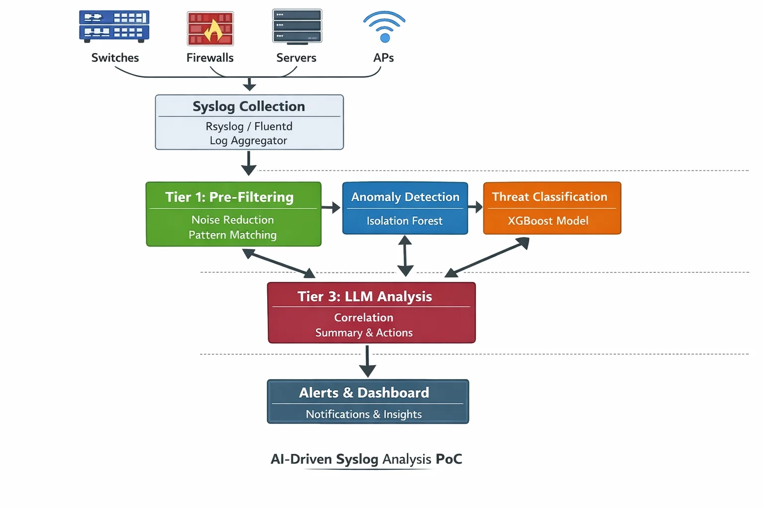
The Full Architecture: How It All Fits Together
Here’s the complete pipeline from device to dashboard:
┌─────────────────────────────────────────────────────────────────┐
│                        NETWORK DEVICES                          │
│  Switches, Firewalls, Routers, APs, Servers, Storage            │
│  Generating syslog, SNMP traps, NetFlow, streaming telemetry    │
└─────────────────────┬───────────────────────────────────────────┘
                      │ UDP/514 (syslog), SNMP traps
                      ▼
┌─────────────────────────────────────────────────────────────────┐
│                    COLLECTION LAYER                              │
│  rsyslog / syslog-ng / Fluentd                                  │
│  Receives, normalizes, timestamps, forwards                     │
│  Throughput: 100,000+ msg/sec on commodity hardware              │
└─────────────────────┬───────────────────────────────────────────┘
                      │ TCP / Kafka protocol
                      ▼
┌─────────────────────────────────────────────────────────────────┐
│                    MESSAGE BROKER                                │
│  Apache Kafka (or Redis Streams for smaller scale)              │
│  Topics: raw_logs, filtered_events, ml_scores, alerts           │
│  Retention: 7 days raw, 90 days filtered                        │
└────┬─────────────────┬──────────────────┬───────────────────────┘
     │                 │                  │
     ▼                 ▼                  ▼
┌──────────┐   ┌──────────────┐   ┌──────────────┐
│  TIER 1  │   │   TIER 2     │   │   TIER 3     │
│ Mechani- │   │ ML Models    │   │  LLM Layer   │
│ cal       │   │              │   │              │
│ Filter   │──▶│ • Isolation  │──▶│ • Correlate  │
│          │   │   Forest     │   │ • Explain    │
│ • Regex  │   │ • Prophet    │   │ • Recommend  │
│ • Sever- │   │ • XGBoost    │   │ • Summarize  │
│   ity    │   │ • LSTM       │   │              │
│ • Rules  │   │              │   │ Claude Haiku │
│          │   │ scikit-learn │   │ or local LLM │
│ ~99.97%  │   │ ~80% of      │   │              │
│ dropped  │   │ remaining    │   │ ~50 events/  │
│          │   │ scored/routed│   │   minute      │
└──────────┘   └──────────────┘   └──────────────┘
                                         │
                                         ▼
                              ┌──────────────────┐
                              │   OUTPUT LAYER    │
                              │                   │
                              │ • Slack/PagerDuty │
                              │ • Dashboard       │
                              │ • Auto-remediation│
                              │ • Incident ticket │
                              └──────────────────┘
The beautiful thing about this architecture is that every component is independently scalable. Getting more syslog than your filter can handle? Spin up another filter instance. ML models becoming a bottleneck? Add another worker consuming from the Kafka topic. The LLM tier is the cheapest to scale because it’s processing the least data.
The POC: Building This With a Unix Box and a Few Devices
Alright, enough theory. Let’s build one. Here’s a concrete lab setup you could have running by the weekend.
Hardware
Lab Setup — Minimum Viable POC
═══════════════════════════════

1× Linux box (your "AI server")
   - Any modern x86_64 with 16GB+ RAM
   - Ubuntu 22.04 or Debian 12
   - Could literally be an old desktop
   - If you want local LLM: add a GPU (even a used RTX 3060 works)
   - If you're using Claude API: GPU not needed

3-5× Network devices that generate syslog
   - Managed switches (Cisco, Aruba, Juniper — anything with syslog)
   - A firewall (pfSense on a spare box works great)
   - A Linux server (generates auth.log, kern.log, etc.)
   - Even a Raspberry Pi running services will generate useful logs

Network
   - All devices configured to send syslog to the Linux box
   - SNMP enabled on managed devices for metric polling
Step 1: Set Up the Syslog Receiver
# On your Linux box — install and configure rsyslog
sudo apt update && sudo apt install -y rsyslog

# Enable UDP and TCP syslog reception
sudo tee /etc/rsyslog.d/10-remote.conf << 'EOF'
# Listen for syslog on UDP 514 and TCP 514
module(load="imudp")
input(type="imudp" port="514")

module(load="imtcp")
input(type="imtcp" port="514")

# Template: write logs as JSON for easy parsing
template(name="json-syslog" type="list") {
    constant(value="{")
    constant(value="\"timestamp\":\"") property(name="timereported" dateFormat="rfc3339")
    constant(value="\",\"host\":\"")   property(name="fromhost-ip")
    constant(value="\",\"hostname\":\"") property(name="hostname")
    constant(value="\",\"severity\":") property(name="syslogseverity")
    constant(value=",\"facility\":\"") property(name="syslogfacility-text")
    constant(value="\",\"tag\":\"")    property(name="syslogtag")
    constant(value="\",\"message\":\"") property(name="msg" format="jsonf")
    constant(value="\"}\n")
}

# Write all remote logs to a JSON file AND forward to a named pipe
if $fromhost-ip != "127.0.0.1" then {
    action(type="omfile" file="/var/log/remote/all.json" template="json-syslog")
    action(type="ompipe" pipe="/var/log/remote/syslog.pipe" template="json-syslog")
}
EOF

# Create the log directory and named pipe
sudo mkdir -p /var/log/remote
sudo mkfifo /var/log/remote/syslog.pipe

# Restart rsyslog
sudo systemctl restart rsyslog
Step 2: Configure Your Devices to Send Syslog
! Cisco IOS — send syslog to your Linux box
configure terminal
logging host 10.0.1.100 transport udp port 514
logging trap informational
logging source-interface Vlan1
logging on
end

# pfSense — Status > System Logs > Settings
# Remote Logging: Enable
# Remote log servers: 10.0.1.100:514
# Log everything, or at minimum: firewall events, system events
Step 3: Set Up Kafka (or Redis Streams for Simplicity)
For a POC, Redis Streams is simpler than Kafka and handles lab-scale volumes easily:
# Install Redis
sudo apt install -y redis-server
sudo systemctl enable redis-server

# Verify it's running
redis-cli ping
# Output: PONG

# Create streams (they auto-create on first write,
# but let's set retention)
redis-cli CONFIG SET stream-node-max-entries 10000
Step 4: The Syslog-to-Stream Bridge
#!/usr/bin/env python3
"""
syslog_bridge.py — Reads syslog from named pipe, applies Tier 1
filtering, pushes survivors to Redis Streams.
"""

import json
import re
import redis
import sys

r = redis.Redis(host='localhost', port=6379, decode_responses=True)

# Tier 1 filter patterns (customize for your environment)
DROP_PATTERNS = [
    r"last message repeated \d+ times",
    r"CRON\[\d+\]",                    # Cron job logs
    r"systemd\[\d+\]: Started Session", # Session spam
    r"LINEPROTO.*changed state to up",  # Flap recovery
    r"SEC_LOGIN-5-LOGIN_SUCCESS",       # Normal logins
    r"sshd.*Accepted password",         # Successful SSH
]

ESCALATE_PATTERNS = [
    (r"LINK-3-UPDOWN.*down", "link_down"),
    (r"DUAL-5-NBRCHANGE.*down", "routing_neighbor_down"),
    (r"sshd.*Failed password", "auth_failure"),
    (r"Out of memory", "oom_kill"),
    (r"temperature.*critical", "thermal_critical"),
    (r"PLATFORM.*PWRSPLY.*fail", "power_failure"),
    (r"disk.*error|I/O error", "disk_error"),
    (r"kernel.*segfault", "segfault"),
]

def process_line(line: str):
    try:
        event = json.loads(line.strip())
    except json.JSONDecodeError:
        return

    msg = event.get('message', '')

    # Drop known noise
    for pattern in DROP_PATTERNS:
        if re.search(pattern, msg, re.IGNORECASE):
            r.incr('stats:dropped')
            return

    # Check for escalation patterns
    category = 'unclassified'
    escalate = False
    for pattern, cat in ESCALATE_PATTERNS:
        if re.search(pattern, msg, re.IGNORECASE):
            category = cat
            escalate = True
            break

    # Also escalate anything severity 0-3 (emergency through error)
    if event.get('severity', 7) <= 3:
        escalate = True

    event['category'] = category
    event['escalate'] = escalate

    # Push to Redis Stream
    stream = 'events:escalated' if escalate else 'events:filtered'
    r.xadd(stream, {'data': json.dumps(event)}, maxlen=50000)
    r.incr('stats:passed')

# Read from named pipe
print("Syslog bridge running. Waiting for messages...")
with open('/var/log/remote/syslog.pipe', 'r') as pipe:
    for line in pipe:
        process_line(line)
Step 5: The ML Scoring Engine
#!/usr/bin/env python3
"""
ml_scorer.py — Consumes filtered events from Redis,
runs them through ML models, publishes scored results.
"""

import json
import time
import redis
import numpy as np
from sklearn.ensemble import IsolationForest
from collections import defaultdict, deque

r = redis.Redis(host='localhost', port=6379, decode_responses=True)

# ──────────────────────────────────────────────
# Feature extraction: turn log events into numbers
# ──────────────────────────────────────────────

class FeatureEngine:
    """
    Maintains rolling windows of events and extracts
    numerical features for ML models.
    """
    def __init__(self, window_seconds=60):
        self.window = window_seconds
        self.events = deque()
        self.host_counts = defaultdict(int)
        self.category_counts = defaultdict(int)

    def add_event(self, event: dict):
        now = time.time()
        self.events.append((now, event))
        self.host_counts[event.get('host', 'unknown')] += 1
        self.category_counts[event.get('category', 'unknown')] += 1

        # Purge old events outside the window
        while self.events and self.events[0][0] < now - self.window:
            _, old = self.events.popleft()
            host = old.get('host', 'unknown')
            self.host_counts[host] = max(0, self.host_counts[host] - 1)

    def extract_features(self) -> np.ndarray:
        """
        Returns: [event_rate, unique_hosts, avg_severity,
                  error_ratio, auth_failure_count, link_down_count,
                  hour_of_day, day_of_week]
        """
        now = time.time()
        lt = time.localtime(now)

        total = len(self.events)
        unique_hosts = len([h for h, c in self.host_counts.items() if c > 0])

        severities = [e.get('severity', 5) for _, e in self.events]
        avg_sev = np.mean(severities) if severities else 5.0

        errors = sum(1 for _, e in self.events if e.get('severity', 5) <= 3)
        error_ratio = errors / max(total, 1)

        auth_fails = self.category_counts.get('auth_failure', 0)
        link_downs = self.category_counts.get('link_down', 0)

        return np.array([
            total,                    # events in window
            unique_hosts,             # unique source hosts
            avg_sev,                  # average severity
            error_ratio,              # fraction that are errors
            auth_fails,               # auth failures in window
            link_downs,               # link down events in window
            lt.tm_hour,               # hour of day (0-23)
            lt.tm_wday,               # day of week (0-6)
        ])

# ──────────────────────────────────────────────
# Model setup
# ──────────────────────────────────────────────

# Phase 1: Collect baseline data (first 7 days)
# Phase 2: Train model and score in real time
# The model retrains weekly on accumulated normal data

engine = FeatureEngine(window_seconds=60)
baseline_data = []
model = None
BASELINE_SAMPLES = 10080  # 1 sample per minute × 7 days

print("ML scorer running. Collecting baseline...")

last_sample = 0
last_id = '0-0'

while True:
    # Read new events from Redis Stream
    results = r.xread(
        {'events:escalated': last_id},
        count=100,
        block=5000  # Wait up to 5 seconds
    )

    for stream, messages in (results or []):
        for msg_id, data in messages:
            last_id = msg_id
            event = json.loads(data['data'])
            engine.add_event(event)

    # Extract features every 60 seconds
    now = time.time()
    if now - last_sample >= 60:
        last_sample = now
        features = engine.extract_features()

        if model is None:
            # Still collecting baseline
            baseline_data.append(features)
            remaining = BASELINE_SAMPLES - len(baseline_data)
            if remaining <= 0:
                # Train the model
                X = np.array(baseline_data)
                model = IsolationForest(
                    n_estimators=200,
                    contamination=0.02,
                    random_state=42,
                )
                model.fit(X)
                print(f"Model trained on {len(baseline_data)} samples")
            elif remaining % 1000 == 0:
                print(f"Baseline: {len(baseline_data)}/{BASELINE_SAMPLES}")
        else:
            # Score the current window
            score = model.decision_function(features.reshape(1, -1))[0]
            prediction = model.predict(features.reshape(1, -1))[0]

            result = {
                'timestamp': time.time(),
                'anomaly_score': float(score),
                'is_anomaly': bool(prediction == -1),
                'features': {
                    'event_rate': float(features[0]),
                    'unique_hosts': int(features[1]),
                    'avg_severity': float(features[2]),
                    'error_ratio': float(features[3]),
                    'auth_failures': int(features[4]),
                    'link_downs': int(features[5]),
                },
            }

            # Publish scores
            r.xadd('ml:scores', {'data': json.dumps(result)}, maxlen=10000)

            if result['is_anomaly']:
                r.xadd('alerts:anomaly', {'data': json.dumps(result)}, maxlen=1000)
                print(f"⚠ ANOMALY detected: score={score:.3f} "
                      f"rate={features[0]:.0f} hosts={features[1]:.0f}")
Step 6: The LLM Analysis Layer
#!/usr/bin/env python3
"""
llm_analyst.py — Consumes anomaly alerts and escalated events,
uses an LLM to generate human-readable analysis.
"""

import json
import time
import redis
from anthropic import Anthropic

r = redis.Redis(host='localhost', port=6379, decode_responses=True)
client = Anthropic()

# Collect events for batch analysis (every 5 minutes or on anomaly)
event_buffer = []
last_analysis = time.time()
ANALYSIS_INTERVAL = 300  # 5 minutes

last_anomaly_id = '0-0'
last_event_id = '0-0'

def run_analysis(events: list, anomaly: dict = None):
    if not events and not anomaly:
        return

    context = {
        'events': events[-50:],  # Last 50 events max
        'anomaly_alert': anomaly,
        'timestamp': time.strftime('%Y-%m-%d %H:%M:%S'),
    }

    response = client.messages.create(
        model="claude-haiku-4-5-20251001",
        max_tokens=1024,
        system="""You are a network operations analyst reviewing
        pre-filtered infrastructure events. These have already passed
        through severity filtering and ML anomaly detection.

        For each analysis:
        1. Identify the most significant events
        2. Look for correlations (multiple devices, same timeframe,
           same failure type)
        3. Suggest probable root cause
        4. Recommend specific actions

        Be concise. Network engineers don't want essays.
        Lead with what matters most.""",
        messages=[{
            "role": "user",
            "content": json.dumps(context, indent=2)
        }]
    )

    analysis = response.content[0].text

    # Store the analysis
    r.xadd('analysis:results', {
        'analysis': analysis,
        'event_count': len(events),
        'has_anomaly': bool(anomaly),
        'timestamp': time.time(),
    }, maxlen=5000)

    print(f"\n{'='*60}")
    print(f"ANALYSIS ({len(events)} events)")
    print(f"{'='*60}")
    print(analysis)
    print(f"{'='*60}\n")

print("LLM analyst running. Waiting for events...")

while True:
    # Check for anomaly alerts (high priority)
    anomaly_results = r.xread(
        {'alerts:anomaly': last_anomaly_id},
        count=1,
        block=1000,
    )

    for stream, messages in (anomaly_results or []):
        for msg_id, data in messages:
            last_anomaly_id = msg_id
            anomaly = json.loads(data['data'])
            # Immediate analysis on anomaly
            run_analysis(event_buffer.copy(), anomaly)
            event_buffer.clear()
            last_analysis = time.time()

    # Collect escalated events
    event_results = r.xread(
        {'events:escalated': last_event_id},
        count=50,
        block=1000,
    )

    for stream, messages in (event_results or []):
        for msg_id, data in messages:
            last_event_id = msg_id
            event = json.loads(data['data'])
            event_buffer.append(event)

    # Periodic analysis even without anomalies
    if time.time() - last_analysis >= ANALYSIS_INTERVAL and event_buffer:
        run_analysis(event_buffer.copy())
        event_buffer.clear()
        last_analysis = time.time()
Step 7: Start It Up
# Terminal 1 — Syslog bridge (Tier 1 filter)
python3 syslog_bridge.py

# Terminal 2 — ML scorer (Tier 2 anomaly detection)
python3 ml_scorer.py

# Terminal 3 — LLM analyst (Tier 3 natural language)
python3 llm_analyst.py

# Terminal 4 — Watch the stats
watch -n 1 'redis-cli mget stats:dropped stats:passed'

# Terminal 5 — Read the analysis stream
redis-cli XREAD BLOCK 0 STREAMS analysis:results $
That’s the entire pipeline. Five Python files, one Redis instance, and rsyslog. On a single machine. No Kubernetes. No Kafka cluster. No enterprise license.
What Each Tier Actually Costs to Run
POC Cost Breakdown
═══════════════════

Hardware (one-time):
  Linux box (reuse old hardware):         $0
  Or: used Dell Optiplex on eBay:         $100-200
  Network devices (you probably have some): $0

Software (all open source):
  Ubuntu/Debian:                          $0
  rsyslog:                                $0
  Redis:                                  $0
  Python + scikit-learn + Prophet:        $0
  Anthropic API (Claude Haiku):           ~$0.50/day at lab scale

Monthly operating cost:
  Electricity for one box:                ~$10-15
  Claude Haiku API:                       ~$15/month (generous estimate)
  Total:                                  ~$25-30/month

Compare to:
  Splunk (500MB/day):                     $1,800/year minimum
  Datadog Log Management:                 $0.10/GB ingested + $1.70/M analyzed
  SolarWinds Log Analyzer:                $1,500+ for first node
The Models Aren’t LLMs — And That’s the Point
I want to hammer this home because it’s the thing I found most surprising in my research. The ML models at Tier 2 are nothing like ChatGPT. You can’t talk to them. They don’t understand language. They’re mathematical functions that take arrays of numbers as input and produce numbers as output.
What an LLM does:
  Input:  "Is this log message concerning?"
  Output: "Based on the severity and context, this appears to be..."

What an isolation forest does:
  Input:  [45.0, 12, 5.1, 0.02, 0, 0, 2, 1]
  Output: -0.34

What Prophet does:
  Input:  A column of dates and a column of numbers
  Output: A column of predicted future numbers

What XGBoost does:
  Input:  [847, 23, 1, 3, 1, 0, 8400, 0, 2]
  Output: 0.97 (probability this is a threat)
These models are fast. An isolation forest scores a data point in microseconds. Prophet makes a prediction in milliseconds. XGBoost classifies in microseconds. They don’t need GPUs (though GPUs can help for training on large datasets). They run on CPUs. They use megabytes of RAM, not gigabytes.
And here’s the crucial insight: they don’t need human-designed thresholds. The isolation forest doesn’t need you to tell it “alert at 85% CPU.” It figures out what’s normal from your data. Different networks have different normals. A university network at 2 AM looks nothing like a hospital network at 2 AM. Static thresholds are a one-size-fits-none approach. ML models adapt to your specific environment.
Does this eliminate the need for humans? No. Humans still design the feature engineering (what numbers to feed the model). Humans still label the training data for classification models. Humans still review and act on the alerts. But the models automate the pattern recognition that currently requires a senior engineer staring at screens, which is the most tedious, error-prone, and unsustainable part of the entire operations workflow.
Running Multiple Models on the Same Stream
One of the questions that came up in my research was whether you need to choose between anomaly detection, forecasting, and classification. The answer is: you don’t. They run in parallel.
# All three model types consuming the same event stream
# Each model type has its own consumer group in Redis

# Consumer group 1: Anomaly detection
# Reads events → extracts features → scores → publishes to ml:anomaly

# Consumer group 2: Time series forecasting
# Reads events → aggregates metrics hourly → forecasts → publishes to ml:forecast

# Consumer group 3: Classification
# Reads events → extracts event features → classifies → publishes to ml:classification

# The LLM layer reads from ALL THREE output streams
# and synthesizes a unified analysis
This is the “fan-out” pattern in streaming architectures. Kafka and Redis Streams both support it natively with consumer groups. Each model gets its own copy of every event, processes it independently, and publishes its results to its own output stream. The LLM layer then reads all the output streams and correlates everything.
Think of it like a hospital emergency room. The triage nurse (Tier 1) decides who gets seen. Then the patient might get blood work (anomaly detection), imaging (forecasting), and a specialist consultation (classification) — all happening in parallel. The attending physician (LLM) reads all the results and makes the final diagnosis.
The Correlation Problem: Why You Need the LLM
The ML models are great at spotting individual anomalies. But they can’t do what a senior network engineer does instinctively: connect the dots across different types of events.
Example: The adjacent floor switch failure.
The isolation forest on each switch independently flags “this switch went down.” Three anomaly alerts fire within 90 seconds. Each one is correct. But none of them knows about the other two.
The LLM reads all three alerts, notices they happened within 90 seconds, cross-references the network topology (which it has access to), realizes these switches are on floors 4, 5, and 6 of the same building, and concludes: “Three switches on adjacent floors failed within 90 seconds. This is consistent with a localized infrastructure event — likely power, cooling, or physical layer. Recommend dispatching facilities to check Building A floors 4-6 for power or environmental issues.”
No ML model can do that alone. The isolation forest doesn’t know about building floors. Prophet doesn’t correlate simultaneous failures. XGBoost classifies individual events, not event clusters. The LLM is the only component that can reason across all the data with contextual knowledge of your environment.
This is where AI actually earns its keep. Not reading raw logs. Not replacing regex. Doing the cognitive work that currently requires a human who has deep institutional knowledge of the network topology, the building layout, the maintenance schedule, and the failure history.
What I’d Do Differently Than ChatGPT Suggested
The ChatGPT conversation I started with gave a solid high-level overview, but it made the whole thing sound like you’d go out and buy Apache Kafka, Apache Flink, deploy Kubernetes clusters, and spin up GPU nodes. That’s the enterprise sales pitch version. Here’s what I’d actually tell someone who wants to understand this stuff:
-
Start with
tail -fand Python. Before you deploy anything, just watch your logs stream by. Build intuition for what “normal” looks like. You’ll be surprised how quickly you start noticing patterns. -
Redis Streams, not Kafka. For a lab or even a mid-size deployment, Kafka is overkill. Redis Streams gives you the same pub/sub semantics with consumer groups, in a tool that fits in 50MB of RAM and requires zero configuration.
-
scikit-learn before TensorFlow. You don’t need deep learning for most infrastructure monitoring. Isolation forests, random forests, and gradient boosting handle 90% of use cases and train in seconds on a CPU.
-
Claude Haiku, not GPT-4. For operational analysis — summarizing events, correlating alerts, generating recommendations — you don’t need the most powerful model. You need one that’s fast and cheap. Haiku at $0.25/million input tokens is 60x cheaper than GPT-4 and plenty smart for this task.
-
Feature engineering is the whole game. The ML models are the easy part. Deciding what numbers to feed them is where the domain expertise lives. A message rate of 500/min means nothing without context. 500/min at 2 AM on a Tuesday for this specific device — that’s a feature with meaning.
“All models are wrong, but some are useful.” — George Box
He said that in 1976 about statistical models. It’s still the most honest thing anyone has said about AI.
Where This Idea Stands
I’ve got the architecture mapped out, the code sketched, and a lab that could run this by next weekend. The pieces are all free, open-source, and battle-tested individually. The novel part is wiring them together into a coherent pipeline where mechanical filtering, ML scoring, and LLM analysis each handle the layer they’re best suited for.
The questions I’m still noodling on:
-
Baseline training period. Seven days feels right for an isolation forest to learn “normal,” but some environments have monthly patterns (month-end batch jobs, quarterly compliance scans). Do you need 30 days of baseline before the model is trustworthy?
-
Model drift. Networks change. New devices get added, traffic patterns shift, new applications launch. How often does the model need retraining? Weekly? Monthly? Or do you use an online learning approach that continuously adapts?
-
The Ollama angle. Could you replace the Claude API call with a local model running on Ollama? A quantized Llama 3 8B model can run on CPU and generates decent operational summaries. That eliminates the API cost entirely but probably reduces the quality of correlation and recommendation.
-
The SNMP convergence. My network monitoring piece covers the metric collection side. This piece covers the log analysis side. In reality, these should be the same system. The ML models should be ingesting both structured metrics (SNMP counters) and unstructured logs (syslog messages) to build a complete picture.
-
Alert routing intelligence. Right now the LLM just prints analysis. In a real system, it should know that a power failure alert goes to facilities, a security event goes to the SOC, and a storage prediction goes to the storage team. That’s a whole routing engine on top of what we’ve built.
The enterprise monitoring industry has been selling two products for decades: “we’ll collect your data” and “we’ll show you dashboards.” The first is a commodity. The second is a crutch for humans who can’t process the raw data. AI doesn’t just make dashboards prettier. It makes them optional. When the system can tell you what’s wrong, why it’s wrong, and what to do about it, in plain English, before you even sit down at your desk — that’s not an incremental improvement on SolarWinds. That’s a different product entirely.
And you can prototype it on a box under your desk for the cost of electricity.
FAQ
Do I need a GPU to run the ML models?
No. The ML models in this architecture — isolation forests, Prophet, XGBoost — all run on CPUs. scikit-learn is CPU-optimized and handles datasets up to millions of rows without breaking a sweat. You’d only need a GPU if you’re training deep learning models (LSTMs, transformers) on very large datasets, or if you want to run a local LLM instead of using an API. For the POC described here, a regular desktop CPU with 16GB of RAM is plenty.
How long does it take to train the anomaly detection model?
The isolation forest trains in seconds to minutes depending on dataset size. With 10,000 samples (about a week of 1-minute windows), training takes under 5 seconds on a modern CPU. Prophet is slightly slower — maybe 10-30 seconds for a 60-day dataset. XGBoost trains in seconds for small datasets. The longest part isn’t training; it’s collecting enough baseline data for the model to learn what “normal” looks like. Plan on 1-2 weeks of data collection before the anomaly detection is useful.
What happens when the model gets it wrong?
It will get things wrong, especially early on. False positives (flagging normal events as anomalies) are more common than false negatives. The practical approach: log every model prediction alongside the actual outcome, review the false positives weekly, and retrain with corrected labels. Over time, the model gets better because it’s learning your specific environment. The LLM layer also acts as a sanity check — it can sometimes recognize that a Tier 2 anomaly alert is actually routine when it has broader context.
Can this replace a SIEM like Splunk or Elastic?
Not directly, and it’s not trying to. A SIEM provides long-term log storage, compliance reporting, forensic search, and often a whole security ecosystem (threat intel feeds, SOAR integration, compliance templates). This architecture handles real-time detection and analysis. The ideal setup runs both: the AI pipeline for real-time intelligence, and a SIEM or log store for historical analysis and compliance. That said, for a small environment that currently has no log analysis, this POC gives you 80% of the value at 0% of the Splunk license cost.
How is this different from what Datadog or New Relic already offer?
Datadog and New Relic do offer anomaly detection features, and they’re solid products. The difference is three-fold: cost (they charge per GB or per host, and it adds up fast), intelligence depth (their anomaly detection is typically per-metric, not cross-domain correlation), and the LLM layer (they show you dashboards, not natural-language analysis with recommended actions). If you’re already paying for Datadog and it’s working, this isn’t necessarily better. But if you’re priced out of Datadog, or if you want deeper AI-driven analysis than their built-in features offer, this architecture gives you a path.
What’s the minimum viable lab to test this?
One Linux machine (even a Raspberry Pi 4 with 8GB RAM), one managed switch that sends syslog, and an internet connection for the Claude API. Install rsyslog, Redis, and Python. Configure the switch to send syslog to the Pi. Run the scripts. You’ll have a working three-tier log analysis pipeline in an afternoon. It won’t be production-ready, but you’ll understand exactly how each layer works and why the architecture is structured this way.